Getting Wild with 800 Lines (of Code)

Taking flat data files (binary and text, courtesy of Sierra Chart) and building continuous futures contracts to export to CSV.

I may have botched the last tutorial, but that’s ok, because this one goes above and beyond. What started as a simple idea turned into an entire set of functions that are going to help us handle data files in quantKit. Am I few days late getting it published? Yep. Is there a reason? Yep.

…

Oh, you want me to excuse my tardiness.

Some of the shit I decided to do was harder than anticipated. Harder? Maybe that’s not the best term. It was more confusing than I anticipated. That doesn’t really do it justice either.

Look, futures contracts are fucking weird. It makes sense once you figure it out, but building continuous contracts stumped me for a while. I also realized that I was using some comparison logic that I wouldn’t be able to use when converting this to a low-level language (I will explain in the code breakdown), so I had to spend some time refactoring those comparisons.

So, yeah. Basically, I just suck. It is what it is. I’ve got it locked in now, and I should be able to plug and play any different type of back adjustment or rollover logic I want.

Let’s not waste to much time here. There is a lot to get into, so let’s do it.

Code can be found here:

GitHub

BLUF

There is over 800 lines of code in this tutorial. It doesn’t use anything outside of the standard library and Numpy. It does import Plotly, but that was just to test that my charts mimiced the charts Sierra Chart built. I built a continuous-futures contract builder that exactly matches Sierra Chart using only raw integers internally, then export a clean, human-readable CSV.

• Load Sierra Chart static files (SCID ticks, DLY daily)

• Resample ticks to 1-minute bars

• Compute volume-based roll dates (YYYYMMDD ints)

• Back-adjust using daily settlements

• Stitch contracts into a continuous series

• Keep time raw: intraday = UTC microseconds; daily = YYYYMMDD

• Filter by start/end using integer comparisons

• Convert to local time only for export/plots

• Export final minute series to data/SC_MES_Minute.csv

Code

I am going to go through this section by section or function by function at points. There is a lot to unpack.

Imports

These are the imports needed for this project. Most of them are standard library import. Numpy is what we use to manage the data (no Pandas) and Plotly is just there for a test.

import os
import numpy as np
from datetime import datetime, timedelta, timezone
from zoneinfo import ZoneInfo
import plotly.graph_objects as go # <- Only needed to test

Constants

There are a lot of constants to define for this project, most of them are structs (look it up) that we need to format our data correctly or read Sierra Chart’s data. Sierra Chart stores it’s intraday data in binary formats, and I like this, so we also define our data structs in a similar way. We also need some time and month-code constants defined to help us later.

# SCID binary formats
HEADER_DTYPE = np.dtype(
    [
        (”FileTypeUniqueHeaderID”, “S4”),
        (”HeaderSize”, “<u4”),
        (”RecordSize”, “<u4”),
        (”Version”, “<u2”),
        (”Unused1”, “<u2”),
        (”UTCStartIndex”, “<u4”),
        (”Reserve”, “S36”),
    ]
)

RECORD_DTYPE = np.dtype(
    [
        (”DateTime”, “<i8”),
        (”Open”, “<f4”),
        (”High”, “<f4”),
        (”Low”, “<f4”),
        (”Close”, “<f4”),
        (”NumTrades”, “<u4”),
        (”TotalVolume”, “<u4”),
        (”BidVolume”, “<u4”),
        (”AskVolume”, “<u4”),
    ]
)

# Our tick struct/format
TICK_DTYPE = np.dtype(
    [
        # raw microseconds since 1899-12-30 (Sierra Chart epoch)
        (”TimeStamp”, “<i8”),
        (”Price”, “<f8”),  # trade price
        (”Volume”, “<f8”),  # trade volume
        (”Bid”, “<f8”),  # bid at time of trade
        (”Ask”, “<f8”),  # ask at time of trade
    ]
)

OHLCV_DTYPE = np.dtype(
    [
        (”TimeStamp”, “<i8”),  # start of bar, raw micros since 1899-12-30 (SC_EPOCH)
        (”Open”, “<f8”),
        (”High”, “<f8”),
        (”Low”, “<f8”),
        (”Close”, “<f8”),
        (”Volume”, “<f8”),
    ]
)

DAILY_DTYPE = np.dtype(
    [
        (”Date”, “<i8”),  # YYYYMMDD
        (”Open”, “<f8”),
        (”High”, “<f8”),
        (”Low”, “<f8”),
        (”Close”, “<f8”),
        (”Volume”, “<i8”),
        (”OpenInterest”, “<i8”),
        (”BidVolume”, “<i8”),
        (”AskVolume”, “<i8”),
    ]
)

# === Time Constants ===

# Sierra Chart epoch (NOT Unix epoch).
# All SCID .scid files store timestamps as 64-bit integers
# representing microseconds since 1899-12-30 00:00:00.
# This matches legacy Excel/Windows serial-date conventions
# and allows handling of historical equities that predate 1970.
SC_EPOCH = datetime(1899, 12, 30)

# Microsecond unit for consistency in conversions
SC_MICROS = np.timedelta64(1, “us”)

# CME month codes
MONTH_CODES = {
    “F”: 1,
    “G”: 2,
    “H”: 3,
    “J”: 4,
    “K”: 5,
    “M”: 6,
    “N”: 7,
    “Q”: 8,
    “U”: 9,
    “V”: 10,
    “X”: 11,
    “Z”: 12,
}

START_DATE = “2024-06-01”
END_DATE = “2025-09-01”

PATH_DIR = r”C:\SierraChart\Data”

Helpers

Anything that I used more than once (or plan to use more than once in the future) became it’s own helper function. Some of these aren’t used in this complete project. They were helpers I used earlier on, but as I refactored the project, I didn’t need them anymore. I left them in there just in case we might need them again in the future.

Roll boundary note. To stitch intraday futures you can’t cut at calendar midnight. CME sessions run 17:00–16:00 Central Time, so a roll date actually flips at 17:00 CT on the prior local day. In this tutorial I approximate that by converting the roll date in UTC and shifting by a fixed 7 hours. This helper is not timezone/DST aware, so the seam is early by 5–6 hours versus CME’s exact 22:00/23:00 UTC boundary. It’s good enough here because both legs are cut at the same point and back-adjustment uses daily settlements, so prices line up and the chart matches visually. For a precise implementation later, I’ll convert “(roll_date − 1) 17:00 America/Chicago → UTC” with DST handling.

def micros_to_dt64(us):
    return SC_EPOCH.astype(”datetime64[us]”) + (us.astype(”<i8”) * SC_MICROS)


def utc_to_local(us: int) -> datetime:
    “”“
    Convert UTC microseconds since Epoch
    into the local time (system timezone) as Python datetime.
    “”“
    # UTC base time
    dt_utc = datetime(1899, 12, 30, tzinfo=ZoneInfo(”UTC”)) \
             + timedelta(microseconds=int(us))

    return dt_utc.astimezone()


def yyyymmdd_to_dt64(val: int) -> np.datetime64:
    s = str(val)
    return np.datetime64(f”{s[:4]}-{s[4:6]}-{s[6:]}”)


def yyyymmdd_to_micros_roll_boundary(date_int: int) -> int:
    “”“
    Convert YYYYMMDD integer to UTC microseconds since Sierra epoch (1899-12-30),
    adjusted to 17:00 UTC of the *previous* day (CME rollover boundary).
    “”“
    # Parse YYYYMMDD to datetime (UTC midnight of that date)
    year = date_int // 10000
    month = (date_int // 100) % 100
    day = date_int % 100
    midnight = datetime(year, month, day)

    # Subtract 7 hours → previous day 17:00 UTC
    roll_time = midnight - timedelta(hours=7)

    # Return microseconds since Sierra epoch
    return int((roll_time - SC_EPOCH).total_seconds() * 1_000_000)


def parse_contract_code(sym: str) -> int:
    “”“
    Parse a futures contract code into YYYYMM integer.
    Handles any root length, just looks at the last 3 chars.

    Example:
        >>> parse_contract_code(”MESH24”)
        202403
        >>> parse_contract_code(”ESU24”)
        202409
    “”“
    code = sym[-3:]  # last three characters: month + 2-digit year
    mon = code[0]
    yy = int(code[1:])

    if mon not in MONTH_CODES:
        raise ValueError(f”Unknown month code: {mon} in {sym}”)

    year = 2000 + yy  # always assume 2000s for now
    month = MONTH_CODES[mon]

    return year * 100 + month


def get_settlement(contract: np.ndarray, roll_date: int) -> float:
    “”“Return the settlement (close) on the last bar before roll_date.”“”
    # Convert entire column of YYYYMMDD ints into datetime64[D]
    dates = contract[”Date”]
    idx = np.searchsorted(dates, roll_date) - 1
    if idx < 0:
        raise ValueError(”No settlement found before roll date.”)
    return contract[”Close”][idx]


def shift_contract(arr: np.ndarray, adj: float):
    “”“Shift OHLC values of a contract by adj (in-place).”“”
    arr[”Open”] += adj
    arr[”High”] += adj
    arr[”Low”] += adj
    arr[”Close”] += adj

Getting contracts

These two functions are how we get the contracts we need for our continuous contracts. They go to a specified directory and return our requested date range contracts by using some of the constants we defined earlier to help. You will see that the discover_contracts function just returns all the contracts with the correct name in the directory and the contracts_in_range function actually returns the correct contracts that we want for our specific request.

def discover_contracts(data_dir: str, root: str):
    “”“
    Find unique contracts for a given root symbol in a directory.

    Scans all filenames starting with the root (e.g. “MES”) and extracts
    contract codes (month+year). Returns sorted unique records.

    Args:
        data_dir (str): Directory containing contract data files.
        root (str): Futures root symbol (e.g. “MES”, “ES”, “CL”).

    Returns:
        list[tuple[int, int, str]]: Sorted unique contracts as (year, month, symbol).

    Example:
        >>> discover_contracts(”/data”, “MES”)
        [(2024, 6, “MESM24”), (2024, 9, “MESU24”)]
    “”“
    root = root.upper()
    seen = set()
    out = []

    for fn in os.listdir(data_dir):
        name = fn.upper()
        if not name.startswith(root):
            continue

        # Extract 3-char contract code (e.g. ‘M24’)
        code = name[len(root): len(root) + 3]
        if len(code) != 3:
            continue

        mon = code[0]
        yy = code[1:]

        # Validate month code and year digits
        if mon not in MONTH_CODES:
            continue
        if not yy.isdigit():
            continue

        sym = f”{root}{mon}{yy}”
        if sym in seen:
            continue
        seen.add(sym)

        # Expand YY into YYYY (assume <70 => 2000s, else 1900s)
        year = 2000 + int(yy) if int(yy) < 70 else 1900 + int(yy)
        month = MONTH_CODES[mon]

        out.append((year, month, sym))

    # Explicit insertion sort by (year, month)
    for i in range(1, len(out)):
        key_item = out[i]
        j = i - 1
        while j >= 0 and (
            out[j][0] > key_item[0]
            or (out[j][0] == key_item[0] and out[j][1] > key_item[1])
        ):
            out[j + 1] = out[j]
            j -= 1
        out[j + 1] = key_item

    return out


def contracts_in_range(data_dir: str, root: str, start: str, end: str):
    “”“
    Slice contracts for a given root symbol within a date range.

    Uses discover_contracts() to build the full contract list, then
    returns only those covering [start, end], including the immediately
    prior contract for rollover/back-adjust purposes.

    Args:
        data_dir (str): Directory containing contract data files.
        root (str): Futures root symbol (e.g. “MES”, “ES”, “CL”).
        start (str): Start date as ‘YYYY-MM-DD’.
        end (str): End date as ‘YYYY-MM-DD’.

    Returns:
        list[str]: Contract symbols covering the date range.

    Example:
        >>> contracts_in_range(”/data”, “MES”, “2024-06-01”, “2024-12-01”)
        [’MESM24’, ‘MESU24’, ‘MESZ24’]
    “”“
    syms = discover_contracts(data_dir, root)
    if not syms:
        return []

    # Convert start to (year, month)
    dt_month = np.datetime64(start, “M”)
    dt_obj = dt_month.astype(object)
    s_y = dt_obj.year
    s_m = dt_obj.month

    # Convert end to (year, month)
    dt_month = np.datetime64(end, “M”)
    dt_obj = dt_month.astype(object)
    e_y = dt_obj.year
    e_m = dt_obj.month

    # Find first contract >= start
    start_idx = len(syms) - 1
    for i, (y, m, _) in enumerate(syms):
        if (y, m) >= (s_y, s_m):
            start_idx = i
            break
    if start_idx > 0:
        start_idx -= 1  # include prior

    # Find last contract <= end
    end_idx = start_idx
    for i, (y, m, _) in enumerate(syms):
        if (y, m) <= (e_y, e_m):
            end_idx = i

    if end_idx < len(syms) - 1:
        end_idx += 1

    # Collect results
    out = []
    for i in range(start_idx, end_idx + 1):
        _, _, sym = syms[i]
        out.append(sym)

    return out

Load daily data

Two functions to get daily data files. Sierra Chart saves these files as basic text files (.dly). These two functions use the contracts list generated by the previous functions to actually load each contract and its data into memory for us to use. We use our DAILY_DTYPE struct to structure the data.

def load_daily_data(path: str) -> np.ndarray:
    “”“
    Load entire daily data file into structured array.

    Args:
        path (str): Path to .dly file (CSV-like SierraChart daily file).

    Returns:
        np.ndarray: Daily records with dtype=DAILY_DTYPE
    “”“
    # Read raw text
    with open(path, “r”) as f:
        lines = f.readlines()

    # Drop header (first line)
    lines = lines[1:]

    out = np.empty(len(lines), dtype=DAILY_DTYPE)

    price_mult = 100.0  # for ES/MES; TODO: detect per-symbol later

    for i, line in enumerate(lines):
        parts = line.strip().split(”,”)

        # Parse YYYY/MM/DD → YYYYMMDD integer
        date_str = parts[0].strip()
        year, month, day = date_str.split(”/”)
        date_int = int(year + month + day)

        out[i][”Date”] = date_int
        out[i][”Open”] = float(parts[1]) / price_mult
        out[i][”High”] = float(parts[2]) / price_mult
        out[i][”Low”] = float(parts[3]) / price_mult
        out[i][”Close”] = float(parts[4]) / price_mult
        out[i][”Volume”] = int(float(parts[5]))
        out[i][”OpenInterest”] = int(float(parts[6]))

        # Some Sierra files may not have bid/ask columns → guard it
        if len(parts) > 7:
            out[i][”BidVolume”] = int(float(parts[7]))
            out[i][”AskVolume”] = int(float(parts[8]))
        else:
            out[i][”BidVolume”] = 0
            out[i][”AskVolume”] = 0

    return out


def load_daily_contracts(data_dir: str, contracts: list[str]) -> dict[str, np.ndarray]:
    “”“
    Load full daily data for multiple contracts.

    Args:
        data_dir (str): Directory with daily files.
        contracts (list[str]): List of contract codes (e.g. [’MESU24’, ‘MESZ24’]).

    Returns:
        dict[str, np.ndarray]: Mapping {contract -> daily data array}
    “”“
    results = {}

    for sym in contracts:
        path = os.path.join(data_dir, f”{sym}_FUT_CME.dly”)

        if not os.path.exists(path):
            print(f”Warning: no daily file for {sym}”)
            continue

        data = load_daily_data(path)

        results[sym] = data

    return results

Load intraday data

Similar to the previous functions, this set gets us our intraday data. Sierra Chart stores these as flat binary files and they don’t have a different data type for ticks versus OHLCV data. So, you have to read the docs to figure a few things out. Well, I had to read the docs. You don’t have to, you can just read my code instead. Anyway, this takes their .scid files and normalizes it into a tick array we defined.

def load_scid_ticks(path):
    “”“
    Load Sierra Chart .scid file into a normalized tick array.

    Args:
        path (str): path to .scid file

    Returns:
        np.ndarray with dtype=TICK_DTYPE
    “”“
    offset = HEADER_DTYPE.itemsize
    filesize = os.path.getsize(path)
    n_records = (filesize - offset) // RECORD_DTYPE.itemsize
    if n_records <= 0:
        return np.empty(0, dtype=TICK_DTYPE)

    # Memory-map the SCID records into a NumPy array.
    #
    # This uses np.memmap to efficiently treat the binary file as an array
    # without reading the entire file into RAM. It’s the Python equivalent of
    # using mmap() or fread() with a struct in C/Zig.
    mm = np.memmap(
        path, dtype=RECORD_DTYPE, mode=”r”, offset=offset, shape=(n_records,)
    )

    price_mult = 100.0  # ES/MES uses 100 multiplier TODO: autodetect this in the future

    # Convert to normalized tick array
    out = np.empty(n_records, dtype=TICK_DTYPE)
    out[”TimeStamp”] = mm[”DateTime”].astype(”<i8”)
    out[”Price”] = mm[”Close”].astype(np.float64) / price_mult
    out[”Volume”] = mm[”TotalVolume”].astype(np.int64)
    out[”Bid”] = mm[”Low”].astype(np.float64) / price_mult
    out[”Ask”] = mm[”High”].astype(np.float64) / price_mult

    return out


def load_scid_contracts(data_dir: str, contracts: list[str]):
    “”“
    Load multiple .scid contracts into tick arrays.

    Args:
        data_dir (str): Directory containing SCID files.
        contracts (list[str]): Contract symbols (e.g. [’MESM24’, ‘MESU24’]).

    Returns:
        dict[str, np.ndarray]: Mapping contract -> tick array.
    “”“
    results = {}

    for sym in contracts:
        # Build file path (Sierra uses suffix like ‘_FUT_CME.scid’)
        path = os.path.join(data_dir, f”{sym}_FUT_CME.scid”)

        if not os.path.exists(path):
            print(f”Warning: {path} not found, skipping”)
            continue
        ticks = load_scid_ticks(path)
        if len(ticks) > 0:
            results[sym] = ticks

    return results

Resample ticks

This function resamples ticks into minute bars. It doesn’t really care about anything other than the timestamps and aggregating them into OHLCV bars for us. It doesn’t care about timezones or anything like that, so it isn’t effected by the time issues I mentioned earlier in our helpers section.

def resample_to_bars(ticks: np.ndarray, minutes: int = 1) -> np.ndarray:
    “”“
    Convert raw tick data into N-minute OHLCV bars.

    Args:
        ticks (np.ndarray): Tick array with fields (TimeStamp, Price, Volume, ...)
        minutes (int): bar length in minutes (default = 1).
            Examples:
                1 -> 1-minute bars
                5 -> 5-minute bars
                240 -> 4-hour bars

    Returns:
        np.ndarray: OHLCV bars with dtype=OHCLV_DTYPE
    “”“
    if ticks.size == 0:
        return np.empty(0, dtype=OHLCV_DTYPE)

    # Floor tick timestampes to start of their minute
    micros_per_bar = minutes * 60 * 1_000_000
    bar_bins = (ticks[”TimeStamp”] // micros_per_bar) * micros_per_bar

    bars = []
    current_bar = bar_bins[0]

    # Init OHLCV from first tick
    o = h = l = c = ticks[”Price”][0]
    v = ticks[”Volume”][0]

    for i in range(1, ticks.size):
        ts = ticks[”TimeStamp”][i]
        price = ticks[”Price”][i]
        vol = ticks[”Volume”][i]
        bar = bar_bins[i]

        if bar == current_bar:
            # Still inside this bar
            if price > h:
                h = price
            if price < l:
                l = price
            c = price
            v += vol
        else:
            # close previous bar
            bars.append((current_bar, o, h, l, c, v))
            # start new bar
            current_bar = bar
            o = h = l = c = price
            v = vol

    # Store last bar
    bars.append((current_bar, o, h, l, c, v))

    return np.array(bars, dtype=OHLCV_DTYPE)

Volume-based rollover

This is where shit got fun. Sierra Chart uses daily data files to determine rollovers. It makes sense. It is a much smaller file and relatively trivial to use. I will do something similar in quantKit. This particular rollover calculation just compares daily volume in contracts and returns a list of rollover dates from contract to contract. It rolls over when volume of the oncoming contract exceeds the daily volume of the current contract. Simple.

def volume_based_rollover(
    contracts: list[str], daily_data: dict[str, np.ndarray]
) -> list[dict]:
    “”“
    Determine rollover dates using Sierra-style volume-based rollover.

    Args:
        contracts (list[str]): Ordered list of contract codes (e.g. [’MESH24’, ‘MESM24’, ...]).
        daily_data (dict): Mapping {contract -> daily bars}, dtype must have
                           fields: (”Date”, “Open”, “High”,
                                    “Low”, “Close”, “Volume”)

    Returns:
        list[dict]: rollover schedule, e.g.
            [{”date”: int, “from”: “MESH24”, “to”: “MESM24”}, ...]
    “”“
    roll = []

    for i in range(len(contracts) - 1):
        front = contracts[i]
        back = contracts[i + 1]

        df = daily_data.get(front)
        dn = daily_data.get(back)
        if df is None or dn is None:
            continue

        # Get expiry year, month from the contract code
        ym = parse_contract_code(front)
        y = ym // 100
        m = ym % 100

        # Restrict to that month/year only
        win_dates = []
        for d in np.intersect1d(df[”Date”], dn[”Date”]):
            s = str(int(d))
            dy, dm = int(s[:4]), int(s[4:6])
            if dy == y and dm == m:
                win_dates.append(int(d))

        rollover_date = None
        for d in sorted(win_dates):
            vol_front = df[df[”Date”] == d][”Volume”][0]
            vol_back = dn[dn[”Date”] == d][”Volume”][0]
            if vol_back > vol_front:
                rollover_date = d
                break

        if rollover_date:
            roll.append(
                {
                    “from”: front,
                    “to”: back,
                    “date”: rollover_date,
                }
            )

    return roll

Back-adjust contracts

The back_adjust_contracts function uses the rollover dates from the previous function (or any other similar rollover function) and calculates back adjustments and returns the adjusted contracts. The daily file already uses the settlement price as its close price. Meaning, it is not the last tick of the day. There is a difference, and this will be something to address in quantKit when I get to it. Not all daily data is built the same.

def back_adjust_contracts(daily_contracts: dict[str, np.ndarray],
                          intraday_contracts: dict[str, np.ndarray] | None,
                          rolls: list[dict]) -> tuple[dict[str, np.ndarray], dict[str, np.ndarray] | None]:
    “”“
    Perform back-adjustment using daily settlements.

    Args:
        daily_contracts (dict): {symbol -> OHLCV array with “Date”}
        intraday_contracts (dict or None): {symbol -> OHLCV array with “TimeStamp”} (optional)
        rolls (list): [{”from”: “H24”, “to”: “M24”, “date”: int}, ...]

    Returns:
        (dict, dict|None): adjusted daily contracts, adjusted intraday contracts
    “”“
    if intraday_contracts is not None:
        adjusted = {sym: arr.copy() for sym, arr in intraday_contracts.items()}
    else:
        adjusted = {sym: arr.copy() for sym, arr in daily_contracts.items()}

    expired = []

    for roll in rolls:  # rolls must be sorted by date
        from_sym = roll[”from”]
        to_sym   = roll[”to”]
        roll_date = roll[”date”]

        # settlement always comes from daily
        old_contract = daily_contracts[from_sym]
        new_contract = daily_contracts[to_sym]

        old_settle = get_settlement(old_contract, roll_date)
        new_settle = get_settlement(new_contract, roll_date)

        diff = new_settle - old_settle

        # All expired contracts get shifted by this new diff
        for sym in expired + [from_sym]:
            if sym in adjusted:
                shift_contract(adjusted[sym], diff)

        expired.append(from_sym)

    return adjusted
 

Stitch contracts

Almost done, y’all.

This function takes all of our contracts and stitches them together at the rollover dates. It doesn’t care whether or not the contracts have been adjusted.

def stitch_contracts(
    contracts: list[str], data: dict[str, np.ndarray], rolls: list[dict]
) -> np.ndarray:
    “”“
    Stitch together multiple contracts into a continuous series using rollover dates.

    Args:
        contracts (list[str]): Ordered list of contract codes.
        data (dict): {contract -> bar array}, bar dtype must include “TimeStamp”.
        rolls (list[dict]): Rollover events [{”from”:, “to”:, “date”:}, ...]

    Returns:
        np.ndarray: Stitched bars, no back adjustment.
    “”“
    stitched = []

    # Build quick lookup for roll dates
    roll_dates = {(r[”from”], r[”to”]): r[”date”] for r in rolls}

    # Detect date/timestamp field
    use_date = “Date” in data[contracts[0]].dtype.names

    for i in range(len(contracts)):
        sym = contracts[i]
        bars = data.get(sym)
        if bars is None or bars.size == 0:
            continue

        # Determine slice window for this contract
        start_date = None
        end_date = None

        # If this contract has an incoming rollover
        if i > 0:
            prev = contracts[i - 1]
            if (prev, sym) in roll_dates:
                start_date = roll_dates[(prev, sym)]

        # If this contract has an outgoing rollover
        if i < len(contracts) - 1:
            nxt = contracts[i + 1]
            if (sym, nxt) in roll_dates:
                end_date = roll_dates[(sym, nxt)]

        # Apply filters
        out = []
        for j in range(bars.shape[0]):
            if use_date:
                # daily: already YYYYMMDD int
                dts = bars[”Date”][j]

                if start_date is not None and dts < start_date:
                    continue
                if end_date is not None and dts > end_date:
                    continue
            else:
                # intraday: convert TimeStamp micros -> date
                ts = bars[”TimeStamp”][j]

                if start_date is not None:
                    start_date_ts = yyyymmdd_to_micros_roll_boundary(start_date)
                else:
                    start_date_ts = None
                
                if end_date is not None:
                    end_date_ts = yyyymmdd_to_micros_roll_boundary(end_date)
                else:
                    end_date_ts = None

                if start_date_ts is not None and ts < start_date_ts:
                    continue
                if end_date_ts is not None and ts > end_date_ts:
                    continue


            out.append(bars[j])

        if out:
            stitched.extend(out)

    if len(stitched) == 0:
        return np.empty(0, dtype=data[contracts[0]].dtype)

    return np.array(stitched, dtype=data[contracts[0]].dtype)

Build contracts wrapper

We made it!

The final piece. This is the wrapper that brings it all together. It returns our finished chart.

def build_continuous_chart(
    root: str,
    data_dir: str,
    start: str,
    end: str,
    chart_type: str = “intraday”,   # “daily” or “intraday”
    interval: int = 1,              # minutes for intraday; ignored if daily
    rollover: str = “volume”,       # only “volume” supported right now
    back_adjust: bool = True
) -> np.ndarray:

    contracts = contracts_in_range(data_dir, root, start, end)

    daily_data = load_daily_contracts(data_dir, contracts)

    if rollover == “volume”:
        rolls = volume_based_rollover(contracts, daily_data)
    else:
        rolls = []

    if chart_type == “daily”:
        bars_by_contract = daily_data
    elif chart_type == “intraday”:
        scid_ticks = load_scid_contracts(data_dir, contracts)
        bars_by_contract = {}
        for sym, ticks in scid_ticks.items():
            bars_by_contract[sym] = resample_to_bars(ticks, minutes=interval)
    else:
        raise ValueError(f”Unknown chart_type: {chart_type}”)
    
    if back_adjust:
        bars_by_contract = back_adjust_contracts(daily_data, bars_by_contract if chart_type==”intraday” else None, rolls)

    stitched = stitch_contracts(contracts, bars_by_contract, rolls)

    final = []
    for i in range(stitched.shape[0]):
        if “Date” in stitched.dtype.names:
            dts = stitched[”Date”][i]
            start_int = int(start.replace(”-”, “”))
            end_int = int(end.replace(”-”, “”))
            if dts < start_int or dts > end_int:
                continue
        else:
            ts = stitched[”TimeStamp”][i]
            start_micros = yyyymmdd_to_micros_roll_boundary(int(start.replace(”-”, “”)))
            end_micros = yyyymmdd_to_micros_roll_boundary(int(end.replace(”-”, “”)))

            if ts < start_micros or ts > end_micros:
                continue
            
        final.append(stitched[i])


    if len(final) == 0:
        return np.empty(0, dtype=stitched.dtype)

    return np.array(final, dtype=stitched.dtype)

Make a damn CSV

The final touch. Let’s make a human-readable CSV.

chart = build_continuous_chart(
    root=”MES”,
    data_dir=PATH_DIR,
    start=”2025-06-01”,
    end=END_DATE,
    chart_type=”intraday”,
    interval=1,
    rollover=”volume”,
    back_adjust=True
)

# ----------------------
# Save to CSV
# ----------------------
if chart.size > 0:
    output_path = os.path.join(”data”, “SC_MES_Minute.csv”)

    # make sure directory exists
    os.makedirs(os.path.dirname(output_path), exist_ok=True)

    if “Date” in chart.dtype.names:
        x_vals = [yyyymmdd_to_dt64(int(d)).item() for d in chart[”Date”]]
        cols = [name for name in chart.dtype.names if name != “Date”]
    else:
        x_vals = [utc_to_local(ts) for ts in chart[”TimeStamp”]]
        cols = [name for name in chart.dtype.names if name != “TimeStamp”]

    export_data = np.column_stack([x_vals] + [chart[name] for name in cols])
    header = “DateTime,” + “,”.join(cols)
    fmt = [”%s”] + [”%.6f”] * (export_data.shape[1] - 1)

    np.savetxt(
        output_path,
        export_data,
        delimiter=”,”,
        fmt=fmt,
        header=header,
        comments=”“
    )

    print(f”✅ Saved: {output_path} ({chart.size} bars)”)
else:
    print(”⚠️ No data to export.”)

And the outcome:

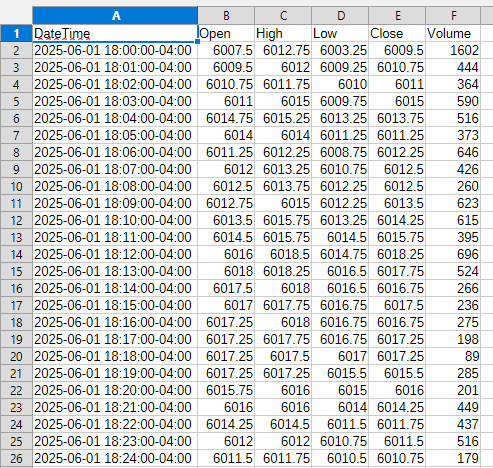
Closing

As you can see, there is a lot of scaffolding here for working with local data files in the future. I like the way Sierra Chart handles local data files without using a database, and I will probably implement something similar for quantKit when it’s time. There is a lot to build from here, and I look forward to adding it into quantKit soon. For now, it’s just a solid tutorial to help you see how you can find, manipulate, and export data for your needs without having to get funky with APIs.

What’s next?

The next post will be a paid post. I am going to create a testing suite for strategies in a spreadsheet. The goal is to have 2-3 strategy ideas in this suite to showcase how it works. I will also build a daily oriented template that will generate orders for daily strategies. This shouldn’t be too difficult to setup, but as we saw from this one, sometimes I misjudge how hard something can be.

Until next time.

Happy hunting.

This post doesn’t represent any type of advice, financial or otherwise. Its purpose is to be informative and educational. Backtest results are based on historical data, not real-time data. There is no guarantee that these hypothetical results will continue in the future. Day trading is extremely risky, and I do not suggest running any of these strategies live.